44 change order of data labels in excel chart
Excel tutorial: How to reverse a chart axis To make this change, right-click and open up axis options in the Format Task pane. There, near the bottom, you'll see a checkbox called "values in reverse order". When I check the box, Excel reverses the plot order. Notice it also moves the horizontal axis to the right. How to Sort Your Bar Charts | Depict Data Studio Here's how you can re-sort the bars within your Microsoft Excel charts: Click on the category labels on the left. You'll see a rectangular border appear around the outside of the categories. Hold your mouse over the lettering, like the word apples. Right-click and select the option on very bottom of the pop-up menu called Format Axis.
Create Dynamic Chart Data Labels with Slicers - Excel Campus Step 6: Setup the Pivot Table and Slicer. The final step is to make the data labels interactive. We do this with a pivot table and slicer. The source data for the pivot table is the Table on the left side in the image below. This table contains the three options for the different data labels.

Change order of data labels in excel chart
Change the plotting order of categories, values, or data series Change the plotting order of data series in a chart Click the chart for which you want to change the plotting order of data series. This displays the Chart Tools. Under Chart Tools, on the Design tab, in the Data group, click Select Data. In the Select Data Source dialog box, in the Legend Entries ... How to create Custom Data Labels in Excel Charts - Efficiency 365 Right click on any data label and choose the callout shape from Change Data Label Shapes option. Now adjust each data label as required to avoid overlap. Put solid fill color in the labels Finally, click on the chart (to deselect the currently selected label) and then click on a data label again (to select all data labels). Is there a way to change the order of Data Labels? Replied on April 4, 2018. Hi Keith, I got your meaning. Please try to double click the the part of the label value, and choose the one you want to show to change the order. Thanks, Rena. -----------------------. * Beware of scammers posting fake support numbers here.
Change order of data labels in excel chart. Format Data Labels in Excel- Instructions - TeachUcomp, Inc. To format data labels in Excel, choose the set of data labels to format. To do this, click the "Format" tab within the "Chart Tools" contextual tab in the Ribbon. Then select the data labels to format from the "Chart Elements" drop-down in the "Current Selection" button group. Then click the "Format Selection" button that ... How to reorder chart series in Excel? - ExtendOffice To reorder chart series in Excel, you need to go to Select Data dialog. 1. Right click at the chart, and click Select Data in the context menu. See screenshot: 2. In the Select Data dialog, select one series in the Legend Entries (Series) list box, and click the Move up or Move down arrows to move the series to meet you need, then reorder them one by one. 3. Excel charts: add title, customize chart axis, legend and data labels Click anywhere within your Excel chart, then click the Chart Elements button and check the Axis Titles box. If you want to display the title only for one axis, either horizontal or vertical, click the arrow next to Axis Titles and clear one of the boxes: Click the axis title box on the chart, and type the text. Sort legend items in Excel charts - teylyn Finally, go back to the data for the helper series up in I2 to I5 and change the values for the helper series to zeros. Now your chart should look like this: step 6. Result: The series order is yellow, blue, pink, green, but the legend items are sorted alphabetically, i.e. apples - pink. bananas - green.
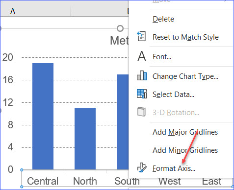
Change order of data labels in chart - Microsoft Community tartan10. Replied on March 4, 2013. In reply to Ty_hell_heaven's post on March 4, 2013. The data were added in the order shown in the list before realizing that the labels could not be moved around. The order of the labels on the right should be, downward, 10, 8, 6, 4, and 2. Report abuse. How to change the Data Label Order in a Column Chart. - Power BI In this scenario, if you want to modify the Legend order, you would need to create separate measures to calculate the results for each type of Business Unit, then place each measure in the Values area in order you wish. For more details, please review this similar thread, it works for column chart. Move and Align Chart Titles, Labels, Legends with the Arrow Keys Select the element in the chart you want to move (title, data labels, legend, plot area). On the add-in window press the "Move Selected Object with Arrow Keys" button. This is a toggle button and you want to press it down to turn on the arrow keys. Press any of the arrow keys on the keyboard to move the chart element. How can I change the order of column chart in excel? Double-click any of the category axis (y-axis) labels. Tick the check box 'Categories in reverse order' in the 'Format Axis' task pane.
Change the Order of Data Series of a Chart in Excel - Excel Unlocked However, to change the order:- Right click on the chart Choose Select Data In the change Source Data Dialog Box, select any one data series Use arrows to shift upward/downward to adjust the order of each data series. Custom Excel Chart Label Positions • My Online Training Hub Custom Excel Chart Label Positions - Setup. The source data table has an extra column for the 'Label' which calculates the maximum of the Actual and Target: The formatting of the Label series is set to 'No fill' and 'No line' making it invisible in the chart, hence the name 'ghost series': The Label Series uses the 'Value ... Change the plotting order of categories, values, or data series Change the plotting order of data series in a chart Click the chart for which you want to change the plotting order of data series. This displays the Chart Tools. Under Chart Tools, on the Design tab, in the Data group, click Select Data. In the Select Data Source dialog box, in the Legend Entries ... Change the labels in an Excel data series | TechRepublic Click the Chart Wizard button in the Standard toolbar. Click Next. Click the Series tab. Click the Window Shade button in the Category (X) Axis Labels box. Select B3:D3 to select the labels in your...

How to Get Colors in Excel Chart Data Lables - Formatting Trick
How to Edit Pie Chart in Excel (All Possible Modifications) Change Data Labels Position Just like the chart title, you can also change the position of data labels in a pie chart. Follow the steps below to do this. 👇 Steps: Firstly, click on the chart area. Following, click on the Chart Elements icon. Subsequently, click on the rightward arrow situated on the right side of the Data Labels option.

Adding rich data labels to charts in Excel 2013 | Microsoft ...
Custom Data Labels with Colors and Symbols in Excel Charts - [How To ... Step 3: Turn data labels on if they are not already by going to Chart elements option in design tab under chart tools. Step 4: Click on data labels and it will select the whole series. Don't click again as we need to apply settings on the whole series and not just one data label. Step 4: Go to Label options > Number.

How to Add Total Data Labels to the Excel Stacked Bar Chart ...
How to Create and Customize a Treemap Chart in Microsoft Excel Simply click that text box and enter a new name. Next, you can select a style, color scheme, or different layout for the treemap. Select the chart and go to the Chart Design tab that displays. Use the variety of tools in the ribbon to customize your treemap. For fill and line styles and colors, effects like shadow and 3-D, or exact size and ...

Enable or Disable Excel Data Labels at the click of a button ...
Data Labels in Excel Pivot Chart (Detailed Analysis) Clicking on any Data labels one time will select all of the Data Labels simultaneously. Then right-click on the Data Table and from the context menu, click on the Format Data Labels. Then in the Format Data Labels, go to the Size and Properties. From there, click on the Text Directions. And from the drop-down menu, click on the Rotate all text 270.

How to change the order of your chart legend - Excel Tips ...
Changing the order of items in a chart - PowerPoint Tips Blog Follow these steps: With the chart selected, click the Chart Tools Design tab. Choose Select Data in the Data section. The Select Data Source dialog box opens. You can only change the values on the left side of the dialog box, so you might have to click the Switch Row/Column button.

How to insert data labels to a Pie chart in Excel 2013
How to add data labels from different column in an Excel chart? This method will guide you to manually add a data label from a cell of different column at a time in an Excel chart. 1. Right click the data series in the chart, and select Add Data Labels > Add Data Labels from the context menu to add data labels. 2. Click any data label to select all data labels, and then click the specified data label to select it only in the chart.

How to Customize Your Excel Pivot Chart Data Labels - dummies
How to Change Excel Chart Data Labels to Custom Values? - Chandoo.org Now, click on any data label. This will select "all" data labels. Now click once again. At this point excel will select only one data label. Go to Formula bar, press = and point to the cell where the data label for that chart data point is defined. Repeat the process for all other data labels, one after another. See the screencast. Points to note:

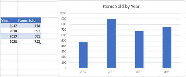
How to Make a Chart in Excel: In 3 Easy Steps - Excel Master ...
Bar chart Data Labels in reverse order - Microsoft Tech Community you're using labels via the "Value from Cells" setting. In this setting a range of cells is specified. The order in which the text appears in these cells is the order that the labels will be displayed. The cells from which the label values are taken are totally independent of the axis order. The first data item gets the first label.

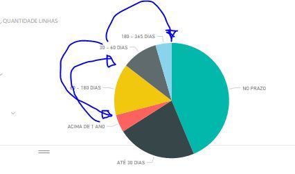
Solved: How to show all detailed data labels of pie chart ...
How to change the order of your chart legend - Excel Tips & Tricks ... Step 1: To reorder the bars, click on the chart and select Chart Tools. Under the Data section, click Select Data. Step 2: In the Select Data Source pop up, under the Legend Entries section, select the item to be reallocated and, using the up or down arrow on the top right, reposition the items in the desired order.

How to make a pie chart in Excel
How to Use Cell Values for Excel Chart Labels - How-To Geek Select the chart, choose the "Chart Elements" option, click the "Data Labels" arrow, and then "More Options." Uncheck the "Value" box and check the "Value From Cells" box. Select cells C2:C6 to use for the data label range and then click the "OK" button. The values from these cells are now used for the chart data labels.

Custom data labels in a chart
Is there a way to change the order of Data Labels? Replied on April 4, 2018. Hi Keith, I got your meaning. Please try to double click the the part of the label value, and choose the one you want to show to change the order. Thanks, Rena. -----------------------. * Beware of scammers posting fake support numbers here.

microsoft excel - Adding data label only to the last value ...
How to create Custom Data Labels in Excel Charts - Efficiency 365 Right click on any data label and choose the callout shape from Change Data Label Shapes option. Now adjust each data label as required to avoid overlap. Put solid fill color in the labels Finally, click on the chart (to deselect the currently selected label) and then click on a data label again (to select all data labels).

Add or remove data labels in a chart
Change the plotting order of categories, values, or data series Change the plotting order of data series in a chart Click the chart for which you want to change the plotting order of data series. This displays the Chart Tools. Under Chart Tools, on the Design tab, in the Data group, click Select Data. In the Select Data Source dialog box, in the Legend Entries ...

excel - How to show series-Legend label name in data labels ...

Dynamically Label Excel Chart Series Lines • My Online ...

Change the format of data labels in a chart

Changing the order of items in a chart

Adding rich data labels to charts in Excel 2013 | Microsoft ...

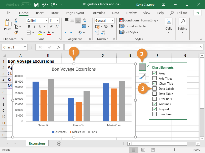
How to Add and Remove Chart Elements in Excel

How to add live total labels to graphs and charts in Excel ...

How to Add Data Labels to an Excel 2010 Chart - dummies

How to add or move data labels in Excel chart?

PCWorld
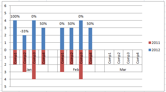
Add % Difference Data Labels to Excel Horizontal Tornado ...

Creating Pie Chart and Adding/Formatting Data Labels (Excel)
Solved: Pie Chart Order of Slices (NOT accordingly to lett ...

Change Chart Data Labels : Chart Data « Chart « Microsoft ...
About Data Labels

excel - VBA Change Data Labels on a Stacked Column chart from ...
Add / Move Data Labels in Charts – Excel & Google Sheets ...
Excel 2013: Charts

Excel charts: add title, customize chart axis, legend and ...

Change the format of data labels in a chart
Adding Data Labels to a Chart (Microsoft Word)

Change the format of data labels in a chart
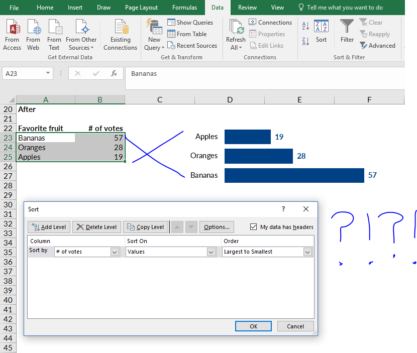
How to Sort Your Bar Charts | Depict Data Studio

Format Number Options for Chart Data Labels in Excel 2011 for Mac
How to Re-order X Axis in a Chart - ExcelNotes

How to Add Data Labels to your Excel Chart in Excel 2013

Display Customized Data Labels on Charts & Graphs
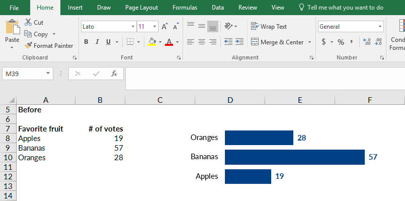
How to Sort Your Bar Charts | Depict Data Studio
How to Add Axis Labels to a Chart in Excel | CustomGuide

Change the format of data labels in a chart

Highlight a Specific Data Label in an Excel Chart - Peltier Tech
Post a Comment for "44 change order of data labels in excel chart"